The study of modern genetics depends on an understanding of the physical and chemical characteristics of DNA. Some of the most fundamental properties of DNA emerge from the features of its four basic building blocks, called nucleotides. Knowing the composition of nucleotides and the differences between the four nucleotides that make up DNA is central to understanding DNA’s role in living systems.

This illustration introduces nucleotide and the terminology used to describe them.

DNA is a nucleotide polymer, or polynucleotide. Each nucleotide contains three components:

1. A five carbon sugar
2. A phosphate molecule
3. A nitrogen-containing base.

The sugar carbon atoms are numbered 1 to 5. The nitrogenous base attaches to base 1, and the phosphate group attaches to base 5. DNA polymers are strings of nucleotides. Cells build them from individual nucleotides by linking the phosphate of one nucleotide to the #3 carbon of another. The repeating pattern of phosphate, sugar, then phosphate again is commonly referred to as the backbone of the molecule.

The sugar in DNA is deoxyribose. Deoxyribose differs from ribose (found in RNA) in that the #2 carbon lacks a hydroxyl group (hence the prefix “Deoxy”). This missing hydroxyl group plays a role in the three-dimensional structure and chemical stability of DNA polymers.

Nucleotides in DNA contain four different nitrogenous bases: Thymine, Cytosine, Adenine, or Guanine. There are two groups of bases:

• Pyrimidines: Cytosine and Thymine each have a single six-member ring.
• Purines: Guanine and Adenine each have a double ring made up of a five-atom ring attached by one side to a six-atom ring.

The order of nucleotides along DNA polymers encodes the genetic information carried by DNA. DNA polymers can be tens of millions of nucleotides long. At these lengths, the four-letter nucleotide alphabet can encode nearly unlimited information.

Nucleosides are similar to nucleotides, except they do not contain a phosphate group. Without this phosphate group, they are unable to form chains.

Test your knowledge of Nucleotides with a quiz

• Illustrations
  • Nucleotides in RNA
  • Complementary Nucleotide Bases
• Problem Sets
  • Nucleotides in DNA practice problems
  • Nucleotides in RNA practice problems
  • Complementary nucleotide bases concept questions

Ribonucleic acids, also called RNA, is the intermediary molecule used by organisms to translate the information in DNA^* to proteins. RNA is also required for DNA replication, regulates gene expression, and can function as an enzyme.

Like DNA, RNA is a polymer - made up of chains of nucleotides^*. These nucleotides have three parts:

1. A five-carbon ribose sugar
2. A phosphate molecule
3. One of four nitrogenous bases: adenine, guanine, cytosine, or uracil

RNA nucleotides form polymers of alternating ribose and phosphate units linked by a phosphodiester bridge between the #3 and #5 carbons of neighboring ribose molecules.

RNA nucleotides differ from DNA nucleotides by a hydroxyl group linked to the #2 carbon of the sugar. This hydroxyl group allows RNA polymers to assume a more diverse number of shapes compared to DNA polymers. The extra hydroxyl group also makes RNA polymers less stable than DNA polymers. The greater variety of shapes RNA polymers form is part of the reason RNA serves more functions than DNA.

Test your understanding of the concepts covered by answering the Nucleotides in RNA practice problems

Video Overview:

• Illustrations
  • Nucleotides in DNA
  • Complementary Nucleotide Bases
• Problem Sets
  • Nucleotides in DNA practice problems
  • Nucleotides in RNA practice problems
  • Complementary nucleotide bases concept questions

DNA^* is the information molecule of the cell. DNA’s capacity to store and transmit heritable information depends on interactions between nucleotide bases and on the fact that some combinations of bases form stable links, while other combinations do not. Base pairs that form stable connections are called complementary bases.

Consistent pairings of complementary bases allow cells to make double-stranded DNA from a single strand template, create messenger RNA from DNA and synthesize proteins from individual amino acids by matching nucleotides bases on messenger RNA with their complementary bases on transfer RNA.

The polynucleotides chains that make up DNA and RNA form via covalent bond^*s between sugar and phosphate subunits of neighboring nucleotides along a chain. In addition to the strong covalent bonds that hold polynucleotide chains together, bases along a polynucleotide chain can form hydrogen bonds with bases on other chains (or with bases elsewhere on the same chain, as with secondary structure in RNA).

The formation of stable hydrogen bonds depends on the distance between two strands, the size of the bases and geometry of each base. Stable pairings occur between guanine and cytosine and between adenine and thymine (or adenine and uracil in RNA). Three hydrogen bonds form between guanine and cytosine. Two hydrogen bonds form between adenine and thymine or adenine and uracil.

Complementary pairs always involve one purine and one pyrimidine base^*. Pyrimidine-pyrimidine pairings do not occur because these relatively small molecules do not get close enough to form hydrogen bonds. Purine-purine links do not form because these bases are too large to fit in the space between the polynucleotide strands. Asymmetry in the structure of non-complimentary purine - pyrimidine pairs cause some crowding and prevent stable bonds from forming.

Take the concept quiz to test your understanding of complementary nucleotide bases.

Video Overview

Related Content

• Illustrations
  • Nucleotides in DNA
  • Nucleotides in RNA
• Problem Sets
  • Nucleotides in DNA practice problems
  • Nucleotides in RNA practice problems
  • Complementary nucleotide bases concept questions

DNA polymerases are the enzymes that replicate DNA in living cells. They do this by adding individual nucleotides to the 3-prime hydroxl group of a strand of DNA. The process uses a complementary, single strand of DNA as a template.

The energy required to drive the reaction comes from cutting high energy phosphate bonds on the nucleotide-triphosphate's used as the source of the nucleotides needed in the reaction.

The illustration above highlights important aspects of the reaction.

DNA polymerases can not create new strands of DNA. They only synthesis double stranded DNA from single stranded DNA. The starting point is a a stretch of single stranded DNA which is double stranded for at least part of its length. In the polymerase chain reaction the double stranded stretch is created by attaching short DNA primers. In living cells, RNA primers are used.

DNA polymerase uses the bases of the longer strand as a template. During strand elongation, two phosphates are cleaved from the incoming nucleotide triphosphate and the resulting nucleotide monophosphate is added to the DNA strand. This results in the:

• Formation of a phosphodiester bond between the phosphate attached to the 5' carbon of the incoming nucleotide and the hydroxyl group on the trailing 3' carbon
• Release of a pyrophosphate molecule
• Extension of the DNA polymer by one nucleotide

Removing two phosphates from the incoming nucleotide and bonding the remaining phosphate to the oxygen on the 3' carbon of the existing strand maintains the repeating sugar-phosphate-sugar-phosphate pattern that makes up the backbone of each DNA polymer.

Orientation of the strand is important. Dependence on energy from the phosphates linked to the 5-prime carbon of the incoming nucleotides means that DNA polymerase can only extend DNA strands by adding nucleotides to the 3-prime end of a DNA strand.

Test your understanding of the concepts covered by this illustration with the DNA Polymerase concept questions.

Video Overview

Related Content

• Illustrations
  • Nucleotides in DNA
  • Nucleotides in RNA
  • Complementary Nucleotide Bases
• Problem Sets
  • Nucleotides in DNA practice problems
  • Nucleotides in RNA practice problems
  • Complementary nucleotide bases concept questions
  • DNA Polymerase concept questions

Genetics is the study of the organization, expression, and transfer of heritable information. The ability for information to pass from generation to generation requires a mechanism. Living organisms use DNA. DNA is a chain, or polymer, of nucleic acids. Individual polymers of DNA can contain hundreds of millions of nucleic acid molecules. These long DNA strands are called chromosomes. The order of the individual nucleic acids along the chain contains information organisms used for growth and reproduction. The use of DNA as the information molecule is a universal property of all life on Earth. Our cellular machinery reads this genetic information allowing our bodies to synthesize the many enzymes and proteins required for life

The illustration explores the relationship between the presence of different alleles at a specific locus and an organism's genotype and phenotype. The organism in the model is a plant. It is diploid, and the trait is flower color. Below is a youtube video demonstrating the use of the illustration anda problem set you can use to test your understanding of these concepts.

Genetic information is carried in discrete units called genes. Each gene contains the information required to synthesize individual cellular components needed for survival. The coordinated expression of many different genes is responsible for an organism's growth and activity.

Within an individual species, genes occur in set locations on chromosomes. This allows their locations to be mapped. The position of a specific gene on a chromosome is called its locus.

Variations in the order of nucleic acids in a DNA molecule allow genes to encode enough information to synthesize the huge diversity of different proteins and enzymes needed for life. In addition to differences between genes, the arrangement of nucleic acids can differ between copies of the same gene. This results in different forms of individual genes. Different forms of a gene are called alleles.

Organisms that reproduce sexually receive one complete copy of their genetic material from each parent. Having two complete copies of their genetic material makes them diploid. Matching chromosomes from each parent are called homologous chromosomes. Matching genes from each parent occur at the same location on homologous chromosomes.

A diploid organism can either have two copies of the same allele or one copy each of two different alleles. Individuals who have two copies of the same allele are said to be homozygous at that locus. Individuals who receive different alleles from each parent are said to be heterozygous at that locus. The alleles an individual has at a locus is called a genotype. The genotype of an organism is often expressed using letters. The visible expression of the genotype is called an organism's phenotype.

Alleles are not created equal. Some alleles mask the presence of others. Alleles that are masked by others are called recessive alleles. Recessive alleles are only expressed when an organism is homozygous at that locus. Alleles that are expressed regardless of the presence of other alleles are called dominant.

If one allele completely masks the presence of another at the same locus, that allele is said to exhibit complete dominance. However, dominance is not always complete. In cases of incomplete dominance, intermediate phenotypes are possible.

Gene interactions can be quite complicated. The example above demonstrates a simple situation in which a single gene corresponds to an individual trait. In more complicated cases, multiple genes can influence an individual trait. This is called polygenic inheritance. In these situations, the relationship between specific alleles and characteristics is not as straightforward.

In his famous pea plant studies, Mendel studied seven traits that have the characteristics needed to allow the observation of inheritance of discrete traits. The traits he studied were seed shape, seed color, flower color, seed pod shape, seed pod color, flower position, and plant stature.

Among the significant contributions of Mendel's work was the understanding that information was passed from one generation to the next in discrete units rather than through blending.

Demonstration video:

• Illustrations
  • Punnett Square
  • Genotype and phenotype probabilities with a monohybrid cross
• Problem Sets
  • Allele, genotype and Phenotype questions
  • Punnett Square Practice Problems
  • Monohybrid genotype and phenotype probability questions

During sexual reproduction, a parent is equally likely to pass on to its offspring either of the two alleles it has at each genetic locus. This makes it possible to list and estimate the probability of specific genotypes being produced from the pairing of two individuals. Given two allele from each parent, four allele combinations are possible. These combinations and their probabilities can be readily visualized using a Punnett square.

To set up a single locus Punnett Square, the genotype of each parent is placed on the sides of a four chambered box. One parent’s alleles are placed across the top. The alleles of the other parent are placed down one side. The alleles on the edges guide how the central squares are filled in. Once complete, a Punnett square shows the genotypes possible from crossing two individuals. Each of the four boxes in the square contains one of the four possible genotypes. The genotype in each box has a 25% probability of occurring every time the two individuals are crossed. If two boxes contain the same genotype, the probability of that genotype occurring doubles to 50%.

Punnett squares are most commonly used to examine genotype probabilities from one genetic locus at a time. They can be used to look at more than one locus at time, but some find the resulting diagrams complicated and difficult to interpret.

The model below illustrates the use of a Punnett Square to determine the possible genotypes that can arise from mating two individuals with known genotypes. The organism in the model is a plant. The plant is diploid. The trait is flower color. Below the illustration is a youtube video demonstrating its use. There is also a problem set you can use to test your understanding of these concepts.

• Illustrations
  • Alleles, genotype and phenotype
  • Genotype and phenotype probabilities with a monohybrid cross
• Problem Sets
  • Allele, genotype and Phenotype questions
  • Punnett Square Practice Problems
  • Monohybrid genotype and phenotype probability questions

Patterns of genetic inheritance obey the laws of probability. In a monohybrid cross, where the allele^*s present in both parents are known, each genotype^* shown in a Punnett Square^* is equally likely to occur. Since there are four boxes in the square, every offspring produced has a one in four, or 25%, chance of having one of the genotypes shown.

Like flipping a coin, previous matings do not influence the results of subsequent matings. Because of random variation, the actual number of each genotype produced over a series of matings (or crosses) between two individuals will differ slightly from the expected 25% per box.

The illustration above explores how the probabilities predicted by a monohybrid Punnett Square relate to the actual pattern of genotypes and phenotype^*s produced from repeatedly crossing two individuals.

Test your understanding of genotype and phenotype probabilities

Video Overview

Related Content

• Illustrations
  • Alleles, genotype and phenotype
  • Punnett Square
• Problem Sets
  • Allele, genotype and Phenotype questions
  • Punnett Square Practice Problems
  • Monohybrid genotype and phenotype probability questions

Chromosome^*s that both males and females possess in matched sets are called autosome^*s. The X and Y-chromosomes that determine the sex of an individual in mammals follow a different pattern and are called allosome^*s. The genes present on the X and Y-chromosomes are called sex-linked genes. Sex-linked genes on the X-chromosome are X-linked genes. Genes on the Y-chromosome are Y-linked.

Females have two X-chromosomes. Males have one X and one Y-chromosome.

With both an X and a Y-chromosome, males inherit both X and Y-linked traits, while females only inherit X-linked traits. Since males have only one copy of each sex chromosome, they are hemizygous for all sex-linked genes, and they always express the phenotype^* of the allele^* they get. In other words, their phenotypes always match their genotype^*s.

Females get two copies of X-linked genes, demonstrating the more typical dominant-recessive expression patterns of non-sex linked traits.

These patterns cause expression patterns of sex-linked traits to differ between male and female offspring.

The X-chromosome is larger and contains more genes than the Y-chromosome, so most sex-linked traits are X-linked traits.

Wild-type fruit flies have dark red eyes, but there are recessive alleles of this eye color gene (called the white gene) that cause individuals to have white eyes. As a recessive trait, the white eye phenotype is masked by the presence of a wild-type (red encoding) allele. If the white gene were on an autosome, it would exhibit classical Mendelian inheritance patterns . However, the gene is on the X-chromosome, making it an excellent illustration of sex-linked inheritance patterns.

Since this particular gene that controls eye color is on the X-chromosome, females (XX) carry two copies, and males (XY) only carry one. In females, the presence of one dominant red encoding allele (X^W) will produce red eyes even if the individual is heterozygous for the white allele. Females can be:

• Homozygous dominant for the red encoding allele - genotype: X^WX^W; phenotype: red eyes.
• Heterozygous - genotype X^WX^w; phenotype: red eyes.
• Homozygous recessive with two white encoding alleles - genotype X^wX^w; phenotype white eyes.

With only one copy of the X-chromosome, all males are hemizygous for this gene. They have only two options:

Observing the ratio of male and female red and white-eyed individuals produced with reciprocal cross^*es shows the difference between sex-linked and classic Mendelian inheritance patterns. Reciprocal crosses involve crossing true breeding red and white-eyed individuals.

Performing the first reciprocal cross: a true-breeding red-eyed female (homozygous dominant) with a true-breeding white-eyed male (hemizygous recessive) results in an F1 generation comprised entirely of red-eyed individuals. 100% of the F1 generation having red-eyes is consistent with what would be predicted based on Mendelian inheritance of a recessive allele. However, with an X-linked gene, the reason for red eyes differs between males and females.

All the female offspring are heterozygous, receiving an X-chromosome with a red allele from their mother and an X-chromosome with the white allele from their father. The presence of the red allele from the mother masks the white allele. Male offspring only have one X-chromosome, which they received from their female parent. Since the female parent is homozygous, whichever allele the males get, they will receive a red-eye allele.

Females are red-eyed because the presence of the recessive copy is masked. Males are red-eyed because they only have one copy of the gene, and that copy is for the red allele.

The females’ phenotype and genotype are consistent with the patterns discovered by Mendel, but the males, as hemizygotes, are not.

The differences between the sexes become more apparent in a cross using the red-eyed F1 male and red-eyed F1 females. This cross produces a 3:1 ratio of red-eyed to white-eyed individuals, but all white-eyed individuals are male. No females have white eyes because they received one of their X-chromosomes from their hemizygous dominant, red-eyed father. The male offspring all received their single X-chromosome from the heterozygous female parent, so half received a red allele, and half received a white allele.

Inheritance patterns with the other reciprocal cross (homozygous recessive female with hemizygous dominant male) diverge from the Mendelian pattern more quickly. The F1 generation contains an equal proportion of white and red-eyed individuals, but all males have white eyes, and all females have red eyes.

Crossing these F1’s again results in a 1:1 ratio of red and white-eyed individuals, but in the F2, half the female offspring and half the male offspring have red eyes.

In both reciprocal crosses, patterns of inheritance beyond the F2 generation vary depending on which F2 individuals are chosen for the cross.

X-linked recessive phenotypes are more commonly observed in males because males are hemizygous for sex-linked traits. Females can be heterozygous for a trait and therefore carry the recessive allele without expressing it. These carrier females have a 50% chance of passing the recessive alleles to their male offspring. These male offspring can not be carriers. If they receive the recessive allele, they will express the recessive trait.

Females expressing detrimental recessive traits like Hemophilia are particularly rare because the only way for a female to be more than a carrier is for a female carrier to produce a daughter with an affected male. The extreme case of an affected female mating with an affected male produces 100% affected offspring.

Test your understanding of the patterns discussed above with the x-linked gene fill in the blank and multiple choice questions

• Illustrations
  • Punnett Square
  • Genotype and phenotype probabilities with a monohybrid cross
  • Punnett Square Calculator
• Problem Sets
  • Punnett Square Practice Problems
  • Genotype and phenotype probability questions
  • X-linked inheritance fill in the blank and multiple choice questions

The Hardy-Weinberg equation describes allele frequencies in populations. It predicts the future genetic structure of a population the way that Punnett Squares predict the results of an individual cross. The equation calculates allele frequencies in non-evolving populations. It is based on the observation that in the absence of evolution, allele frequencies in large randomly breeding populations remain stable from generation to generation.

In real populations, evolution does occur and allele frequencies vary over time. This divergence between real, evolving populations and theoretical, non-evolving populations allows the Hardy-Weinberg equation to be used to explore the effect of evolution on populations. Two major factors that cause real populations to diverge from the equilibrium predicted by the Hardy-Weinberg equilibrium are genetic drift and natural selection.

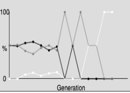
The following illustration shows changes in actual allele frequencies over time compared to the stable structure predicted by the Hardy-Weinberg equation.

Genetic drift is the random variation that results in specific individuals producing more or less offspring than predicted by chance alone. This is most pronounced in small populations and is a major reason real allele frequencies do not remain at Hardy-Weinberg equilibrium values. Genetic drift is random and as such does not result in populations becoming more adapted to their environment.:

Natural selection increases the frequency of a favored allele over another and can cause significant departures from Hardy-Weinberg equilibrium.

Assuming a trait controlled by two alleles where p is the frequency of one allele and q is the frequency of the other allele, the sum of the frequencies must equal 1:

p + q = 1

Given p and q, the Hardy-Weinberg equation is:

The relationship between allele frequencies and genotype frequencies in populations at Hardy-Weinberg Equilibrium is usually described using a trait for which there are two alleles present at the locus of interest.

This calculator demonstrates the application of the Hardy-Weinberg equations to loci with more than two alleles. Visit the genetic drift and selection illustration for more on the Hardy-Weinberg Equilibrium.

Update the values by changing the allele frequency in the blue box below the graph. The calculator has a check that prevents the allele frequencies from summing to any value other than 1. To avoid having your values changed, make sure your values sum to one and enter them from top to bottoms (p then q then r ...)

Number of genotypes for a given number of alleles Given n alleles at a locus, the number genotypes possible is the sum of the integers between 1 and n:

• With 2 alleles, the number of genotypes is 1 + 2 = 3
• 3 alleles there are 1 + 2 + 3 = 6 genotypes
• 4 alleles there are 1 + 2 + 3 + 4 = 10 genotypes.

The general formula for finding the sum of a set of integers from 1 to n is:

Genotypes = n * n+1 / 2

The calculator does not go beyond 5 alleles and 15 possible genotypes. However, the equation above can be used to calculate the number of genotypes for a locus with any number alleles.

If a population has 10 alleles for a specific gene, the combined, total number of homozygous and heterozygous genotypes present in the population will be:

(10 * 11) / 2 = 55

This breaks down to 10 homozygous genotypes and 45 heterozygous genotypes. The sum of the allele frequencies would still need to equal 1 :

p + q + r + s + t + u + v + w + x + y = 1

As would the sum of the genotype frequencies:

p² + 2pq + 2pr + 2ps + 2pt + 2pu + 2pv + 2pw + 2px + 2py + q² + 2qr + 2qs + 2qt +2qu + 2qv + 2qw + 2qx + 2qy + r² + 2rs + 2rt + 2ru + 2rv + 2rw + 2rx + 2ry + s² + 2st+ 2su + 2sv + 2sw + 2sx + 2sy + t² + 2tu + 2tv + 2tw + 2tx + 2ty + u² + 2uv + 2uw +2ux + 2uy + v² + 2vw + 2vx + 2vy + w² + 2wx + 2wy + x² + 2xy + y² = 1

• Illustrations
  • Drift and Selection
• Problem Sets
  • Population Genetics Practice Problem Set